A simple Machine Learning model for predicting churn users

Introduction

This post showcases a simple use case on how you can build a Machine Learning (ML) model to predict which of our active users are likely to churn. A well implemented Churn Prediction Model is a valuable asset to any company. Bringing new users to your business requires a big effort in marketing both in time and budget. It is way less expensive to retain a user than trying to win over a churn user. If you are able to predict which users are at risk of churning, you can target does users in order to retain them.

Data Exploratory Analisis

Regardless of the problem we are going to solve, the first step in any data analysis journey to build an ML model is always exploring and cleaning your data. Most of the times the dataset you work with has to be prepared and cleaned up in order to start building a model, it may have multiple missing values or columns with the wrong data types. This preprocess can take a lot of time, but since it’s out of the scope of this post and for the sake of simplicity, the dataset which we are going to work with is already clean. So the first step will be importing our data and start exploring it

# Import Libraries
import pandas as pd

# Read the Dataset
df = pd.read_csv('data.csv')
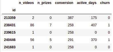
df.head()

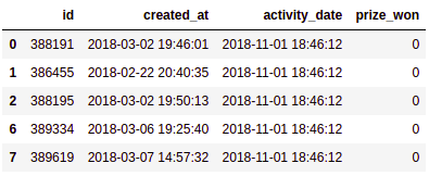
This dataset correspond to the rendering of a webpage where users can watch videos, if certain numbers of videos are watched then the user is rewarded with a prize. In reality it has much more than that, but for this sample case is enough to start working with.

The first column (id) is a unique number identifier that represents each user, the second (created_at) is the date the user created the account, the third (activity_date) is the date a video was viewed and the last (prize_won) is a boolean type column that indicates whether that particular video met the goal to win a prize.

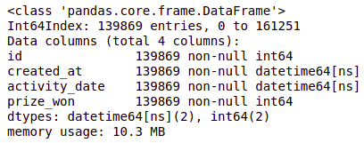
When we explore the DataFrame, we can see that it has more than 130 thousand entries with zero null values, and each column has the correct data type.

df.info()

Since we have multiple entries for the same use, the first step would be to process the DataFrame so that each row corresponds to a specific user. At this point we have to think about what kind of information we can posible extract and could be relevant to build our model. For example, some useful information could be:

Number of videos viewed
Number of prizes won
Conversion days (Number of days between the account creation date and the first video viewed)
Number of active days (Difference between first and las video viewed)
Already Churned?

Let’s start by grouping the users id in order to get some of the information that will allow us to get what we need.

grouped = df1.groupby('id').agg({'created_at':['max'],
                                 'activity_date':['min','max','count'], 
                                 'prize_won':['sum']})
grouped.columns = ['created_at','first_video','last_video', 
                   'n_videos', 'n_prizes']
grouped.reset_index(inplace=True)
grouped.head()

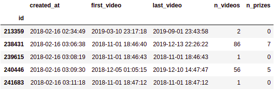
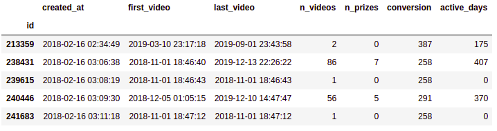
By doing this we have obtained for each user the account creation date, but also the first and last video they watched, the total number of videos viewed and the number of prizes won. Now we need an extra step to obtain the Conversion and active days.

import datetime as dt
grouped['conversion'] = (grouped.first_video - 
                         grouped.created_at).dt.days.astype(int)
grouped['active_days'] = (grouped.last_video - 
                          grouped.first_video).dt.days.astype(int)
grouped.head()

Since the data set we have does not specify whether a user is a churn user or not, we need to define that criteria ourselves. The approach we are going to use is to consider that every user that watched her last video more than 90 days ago is a churn user. So we only need to take the difference between our current day and the last video, and then evaluate if the number is bigger than 90. Finally, we need to retain only the columns with numbers in it because that’s the only data type we can use to build a ML model.

grouped['churn'] = (dt.date.today() - 
                    grouped.last_video.dt.date).dt.days.astype(int)
grouped['churn'] = grouped['churn'].apply(lambda x: 1 if x < 90 else 0)
grouped.drop(columns = ['id','created_at','first_video',
                        'last_video'], inplace = True)
grouped.head()

Now that we have made some preprocessing, we should look closely to the data we have up to this point.

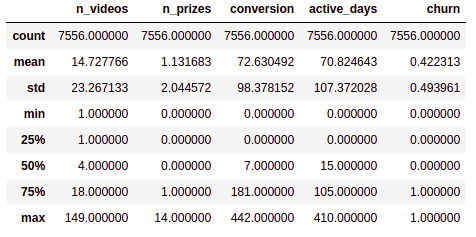
grouped.describe()

As you can see we have almost 8000 entries in our table which is not much, but yet enough to build a simple model. The problem with this table is that the data is very dispersed. In the n_videos columns for example, we have that the 75% of the users have viewed 18 or less videos, while we have a user that have viewed 852 videos, that kind of outliers can lower the accuracy of our model. The same happens in conversion where the mean is around 76 day for a user to convert, while we have some users with near 600 days until conversion. So we need to figure out if we can reduce the number of outliers without losing too much data. For this example, a boxplot may help us identify which rows we can drop.

import matplotlib.pyplot as plt
import seaborn as sns

plt.figure(figsize=(14,10))
sns.set(style="whitegrid")
sns.boxplot(data=grouped.iloc[:,:-1])

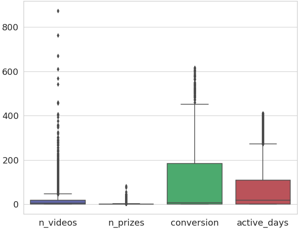
We can see that for the n_videos column we have tons of values outside of our upper fence, if we drop all of them we will lose too much information. So a middle ground would be dropping all users with more than 150 viewed videos. For the conversion column we can see that there are no more outliers after the 450 mark, maybe we can drop all off them without losing too much data. As for the active_days column, is better to leave it as it is. If we drop the rows outside our upper fence, the model may fail in trying to represent our oldest users.

grouped = grouped[(grouped.n_videos < 150) & (grouped.conversion < 450)]
grouped.describe()

Great! We have managed to reduce some of our outliers without losing too much data, now we are left with 7700 entries to train and test our model.

Building the Model

Now that we have the Dataframe clean and ready we have to choose which model is the best to answer our question: “which users are likely to churn?” There are multiple ML models, each one of them has is pros and cons, and are best suited to solve some kind of problems and unable to solve others. It’s our job to figure out which one is the one that perform best to our specific situation.

A churn analysis is a yes or no answer, that kind of problem is called a classification problem. We want to classify each person as a churn user or not. The most known ML models to deal with classification problems are:

Logistic Regression
Naive Bayes
KNN
SVM
Decision Tree
Random Forest

Since this is only a guide, and to avoid going too long, we are going to build only the Random Forest model. But before we do that, we need to split our data. When building a ML model, you use some of your data to train the model, and another part to test it. The proportion you divide your data depends on the amount you have, generally you will take between 75% and 80% to train and the rest to test it. Because our pool is not too big, we will train our model with the 80% of it. To do so we will use the train_test_split method from the sklearn library. This method will randomly divide our data in the proportion we choose.

y = grouped["churn"].values
X = grouped.drop(labels = ["churn"], axis = 1)

from sklearn.model_selection import train_test_split

X_train, X_test, y_train, y_test = train_test_split(X, y, test_size=0.2, random_state=101)

Now that we have our data divided we can train our Random Forest model.

from sklearn.ensemble import RandomForestClassifier
# Instance the method
model = RandomForestClassifier(n_estimators = 300, criterion = "entropy")
# Fit the model to our train data
result = model.fit(X_train, y_train)

We pass two parameters to our model, the first one, “n_estimators”, indicates the number of trees in our forest and the second one, “criterion”, specify which is the criterion he is going to apply to do the split between decisions.

Evaluating the Model

Once that the model has been trained we can test it doing some predictions with our test data.

prediction = model.predict(X_test)

# print the accuracy of the model
from sklearn import metrics
print("accuracy = " , metrics.accuracy_score(y_test, prediction))

accuracy = 0.7466755319148937

Our simple model has a 75% accuracy, not bad!. However, when dealing with classification models, the accuracy it not enough to evaluate the performance of it. Imagine that we are developing a model to predict something that has very low occurrence, say 1%. We can train a model that always fails in predicting that specific event, and it will still have a 99% accuracy because it will be wrong only 1% of the times. So to make a better evaluation of our model, we will introduce 4 new metrics, sensitivity, specificity, precision and F1.

$sensitivity = \frac{TP}{TP + TN}$

$specificity = \frac{TN}{TN + FP}$

$Precision = \frac{TP}{TP + FP}$

$F1 = \frac{Precision*Sensitivity}{Precision + Sensitivity}$

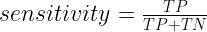
Where TP, TN, FP and FN stands for True Positive, True Negative, False Positive and False Negative respectively . Sensitivity is the ratio between how much were correctly identified as positive to how much were actually positive. Specifity is the ratio between how much were correctly classified as negative to how much was actually negative. Precision is how much were classified as positive out of all positive and finally F1 is the harmonic mean of precision and sensitivity. This final score is a measure of performance of the model’s classification ability and is considered the best indicator of such.

To calculate these metrics we need to obtaining the confusion matrix wich is a table with two rows and two columns that reports the number of FP, TP, FN and TN.

TN, FP, FN, TP = metrics.confusion_matrix(y_test, prediction_rf).ravel()
Sensitivity =  TP / (TP + FN)
print('Sensitivity = ', Sensitivity)
Specificity = TN / (TN + FP)
print('Specificity = ', Specificity)
Precision = TP / (TP + FP)
print('Precision = ', Precision)
F1 = 2 * (Precision * Sensitivity) / (Precision + Sensitivity)
print('F1 = ', F1)

Sensitivity =  0.6497764530551415
Specificity =  0.8224513172966781
Precision =  0.7377326565143824
F1 =  0.6909667194928685

From these metrics we can see that the sensitivity is not as high as the specificity, this means that our model is not as good predicting non churn users as it is predicting churn user, luckily, this is the main goal of our model. Finally the F1 score which is a balance between the precision and sensitivity, is good enough for a first run. Whenever we are facing a classification problem, this is the score we want to maximize in order to improve our model.

Another important result is the relevance of the variables we used to build the model. When higher the value of relevance is, means that it has a stronger correlation with the value we want to predict.

weights = pd.Series(model_rf.feature_importances_,
                    index=X.columns.values)
weights.sort_values(ascending = False)

active_days    0.369124
conversion     0.315415
n_videos       0.223105
n_prizes       0.092356
dtype: float64

In our case, active_days and conversion are the most relevant features then we have n_videos and finally we see that n_prizes has a low correlation. Very low correlation values can sometimes lower the accuracy if our model, so is always important to check weather if all the variables we are considering are important or if we should remove some of them.

What’s next?

So we finally did it, we built a simple model to predict users that are likely to churn. Now what? Well, we can go on and try to improve it, is unlikely that we get the best version of the model in the first run. So we should try to maximize the F1 value.

How do we maximize it? There are multiples approaches we can take: for starters we can try other models or even test the same Random Forest but with different parameters. Perhaps the variables that we are processing are not the most representatives meaning they have a low correlation with the fact that a user is leaving or not.

Once that we are sure of our results and the performance of our model, we should report to the results, talk with you teammates to start planning strategist to retain the users, in this cases the high correlation variables are very important, since it can provide lots of clues about why the users are leaving or in what we should focus to retain them.